Shortest Path Algorithms

Finding the quickest way to get from Point A to Point B is one of the most important problems in computer science.

A. Dijkstra’s Algorithm

Definition:

Dijkstra’s algorithm finds the shortest path from a starting node to all other nodes in a graph with non-negative weights. It is a “Greedy” algorithm.

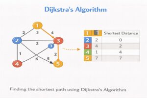
How it Works:

1. Set distance to start node = 0, and all others = Infinity (infty).
2. Use a Priority Queue (Min Heap) to always pick the unvisited node with the smallest known distance.
3. Visit that node and check its neighbors.
4. Relaxation: If you find a shorter path to a neighbor through the current node, update the neighbor’s distance.

Real-World Analogy:

Google Maps: You are at home (Start). You look at all immediate roads. You pick the fastest one. From that new intersection, you again check the fastest connecting roads. You keep doing this, accumulating the time, until you reach the destination.

Complexity: O((V+E) \log V) using a Min Heap.

Limitation: Fails if the graph has negative edge weights (e.g., a “time machine” road that takes -5 minutes).

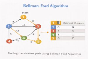
B. Bellman-Ford Algorithm

Definition:

Bellman-Ford also calculates shortest paths but can handle negative edge weights. It is based on Dynamic Programming.

How it Works:

Instead of greedily picking the closest node, Bellman-Ford relaxes all edges repeatedly.

1. If there are V vertices, iterate through all edges V-1 times.
2. For every edge (u, v) with weight w, if distance[u] + w < distance[v], update distance[v].
3. Step 3: Run one more time. If a distance still changes, a Negative Weight Cycle exists (you can spin around forever decreasing cost).

Complexity: O(V \times E). It is slower than Dijkstra.

Comparison: Dijkstra vs. Bellman-Ford