Order of Growth (Best to Worst)

When analyzing algorithms, the overall efficiency is determined by the highest power of $n$, which dictates the function type. The mathematical order of growth from most efficient to least efficient is:

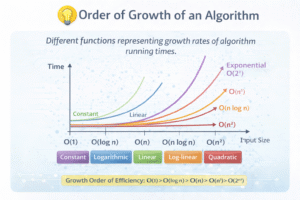
O(1) < O(\log n) < O(n) < O(n \log n) < O(n^2) < O(n^3) < O(2^n) < O(n!)

1. Constant Function

• Time Complexity: O(1)

• Mathematical Form: f(n) = c

• Meaning: The execution time is entirely independent of the input size.

• Algorithm Example: Printing the first element of an array, such as print A[1]. This requires one array access and one print operation, resulting in constant steps.

2. Logarithmic Function

• Time Complexity: O(log n)

• Mathematical Form: f(n) = log n

• Meaning: The input size reduces by a constant factor during each step of the execution.

• Algorithm Example: Binary Search. For an input of $n = 16, the search space halves progressively: 16 ->8 ->4 ->2 ->1 (taking 4 steps).

3. Linear Function

• Time Complexity: O(n)

• Mathematical Form: f(n) = n

• Meaning: The execution time increases directly proportional to the input size.

• Algorithm Example: A single for loop running from 1 to n. If n = 100, the loop runs exactly 100 times.

4. Linearithmic Function

• Time Complexity: O(n log n)

• Mathematical Form: f(n) = n log n

• Meaning: This is a combination of linear work and logarithmic division.

• Algorithm Example: Merge Sort. If n = 8, the calculation is 8 log_2 8 = 8*3 = 24 operations.

5. Quadratic Function

• Time Complexity: O(n^2)

• Mathematical Form: f(n) = n^2

• Meaning: This typically occurs when an algorithm contains two nested loops.

• Algorithm Example: Two for loops iterating from 1 to n. If n = 5, the number of operations is 5*5 = 25.

6. Cubic Function

• Time Complexity: O(n^3)

• Mathematical Form: f(n) = n^3

• Meaning: This occurs when an algorithm relies on three nested loops.

• Algorithm Example: Three for loops iterating from 1 to n. If n = 4, the operations total 4^3 = 64.

7. Polynomial Function

• Mathematical Form: f(n) = n^k \quad (k \ge 1)

• Meaning: This is a broader category that includes linear, quadratic, cubic, etc. Algorithms falling into this category are generally considered “efficient and solvable” in computer science.

• Example: If f(n) = n^4 + n^2 + 10, it simplifies to an order of O(n^4).

8. Exponential Function

• Time Complexity: O(2^n)

• Mathematical Form: f(n) = 2^n

• Meaning: The execution time doubles for every single increment in n.

• Algorithm Example: A naive recursive Fibonacci sequence calculator. For n = 5, it takes 2^5 = 32 operations.

9. Factorial Function

• Time Complexity: O(n!)

• Mathematical Form: f(n) = n!

• Meaning: This represents extremely slow growth and usually occurs when an algorithm tries all possible permutations of an input.

• Algorithm Example: Solving the Traveling Salesman Problem using a brute-force approach. For just n = 5, the operations jump to 5! [cite_start]= 120.

10. Composite / Mixed Function

• Mathematical Form: Equations mixing multiple terms, such as f(n) = n^2 + 5n + 20.

• Simplification: When analyzing these, you drop the lower-order terms and constants, simplifying it to its highest degree, which in this case is O(n^2).