Design Techniques in DSA

Algorithm Design Techniques in DSA

Algorithm design techniques are the foundational blueprints used to solve complex computational problems. Choosing the right technique is essential for writing efficient code, especially when tackling technical interviews or building scalable applications.

Let’s break down three of the most powerful design paradigms: Backtracking, Dynamic Programming (DP), and Divide and Conquer (specifically Merge Sort).

1️⃣ Backtracking (The “Try and Undo” Approach)

Backtracking is a methodical way of trying out different sequences of decisions until you find one that works. It incrementally builds candidates for the solutions and abandons a candidate (“backtracks”) as soon as it determines that the candidate cannot possibly lead to a valid solution.

Simple Analogy: Imagine navigating a complex maze. You walk down a path until you hit a dead end. Instead of starting over from the very beginning, you retrace your steps back to the last intersection (you backtrack) and try a different route.

• How it works:

  1. Choose: Pick an option.

  2. Explore: Recursively move forward with that choice.

  3. Un-choose (Backtrack): If the choice leads to an invalid state, undo the choice and try the next available option.

• When to use it: When you need to find all possible solutions, or when the problem asks for permutations, combinations, or satisfying specific constraints.

• Classic Interview Problems:

  • The N-Queens Problem

  • Sudoku Solver

  • Generating Subsets or Permutations

2️⃣ Dynamic Programming / DP (The “Remember the Past” Approach)

Dynamic Programming is an optimization technique used when a problem can be broken down into overlapping subproblems. Instead of recalculating the same subproblem multiple times (which is highly inefficient), DP solves each subproblem once and stores the answer for future reference.

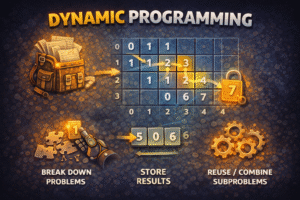
Key Properties Required for DP:

1. Overlapping Subproblems: The problem can be broken down into subproblems which are reused several times.

2. Optimal Substructure: The optimal solution to the main problem can be constructed from the optimal solutions of its subproblems.

The Two DP Approaches:

• Top-Down (Memoization): Start solving the main problem recursively. Whenever you solve a subproblem, store its result in a map or array. Before solving a new subproblem, check if the answer is already stored.

• Bottom-Up (Tabulation): Start solving the smallest subproblems first and iteratively build up to the main problem using a table (usually a 1D or 2D array).

• Classic Interview Problems:

  • Fibonacci Sequence (optimized from O(2n) to $O(n)$)

  • 0/1 Knapsack Problem

  • Longest Common Subsequence

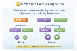
3️⃣ Divide and Conquer (Showcased via Merge Sort)

As we touched on previously, Divide and Conquer splits a problem into independent subproblems, solves them recursively, and combines the results. Merge Sort is the quintessential example of this technique in action.

How Merge Sort applies the paradigm:

1. Divide: The algorithm calculates the middle index and splits the unsorted array into two equal (or roughly equal) halves. This is purely an indexing operation, taking $O(1)$ time.

2. Conquer: It recursively calls Merge Sort on the left half and the right half. It keeps dividing until it reaches the base case: arrays of size 1, which are naturally sorted.

3. Combine (Merge): This is where the actual sorting happens. It takes two sorted sub-arrays and carefully merges them into a single, larger sorted array. This merging process takes linear $O(n)$ time.

• Time Complexity: Always O$(n\log n)$ across worst, average, and best cases.

• Space Complexity: $O(n)$ because it requires auxiliary arrays to hold data during the merging phase.

Quick Comparison Guide

Here is a quick reference table to help identify which technique to use based on the problem characteristics: