Correlation Analysis

What is Correlation Analysis?

Imagine you are looking at two trends in a city over the summer: the number of ice cream cones sold and the number of sunburns reported at the local hospital. You notice that on days when ice cream sales skyrocket, sunburns also go way up.

Are the ice cream cones causing the sunburns? No! They are just connected by a hidden third factor: hot, sunny weather.

In Machine Learning, Correlation Analysis is the process of acting as a matchmaker (or a detective) to see if and how two different columns in your dataset are related to one another. It helps you understand if changing one variable is linked to a change in another.

Connecting to What We Know

Let’s look at our Exploratory Data Analysis (EDA) journey so far:

1. Structure: We checked the foundation (rows, columns, data types, and missing values).
2. Distribution: We looked at single columns in isolation to see their “shape” (like the bell curve of test scores).

Now, we are leveling up. Instead of looking at one column at a time, we are looking at how columns interact with each other.

Why do we care? Because a machine learning model’s entire job is to find relationships. If you want to train a model to predict the price of a house (your target), you need to find out which features (square footage, number of bedrooms, distance to the city) have the strongest mathematical relationship—or correlation—with that price.

Step-by-Step: Understanding Correlation

Here is the logical flow of how data scientists measure these relationships:

1. Finding the Direction

When two variables move together, we want to know which way they are going. There are three possibilities:

• Positive Correlation: When one goes up, the other goes up.

• Example: The size of a house and its price. Bigger houses generally cost more.

• Negative Correlation: When one goes up, the other goes down.

• Example: The age of a used car and its price. As the car gets older, the price usually drops.

• No Correlation (Zero): The variables have nothing to do with each other.

• Example: The color of a car and the driver’s shoe size. It’s just random noise.

2. Measuring the Strength (The ‘r’ Score)

Data scientists don’t just guess; they use math to give this relationship a score. The most common score is called the Pearson Correlation Coefficient, often just written as r.

• The score always lives between -1.0 and 1.0.
• A score of 1.0 is a perfect positive relationship (they move up in exact lockstep).
• A score of -1.0 is a perfect negative relationship (they move in exact opposite directions).
• A score of 0.0 means no relationship at all.

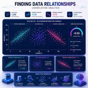
3. Visualizing with Scatter Plots

The easiest way to understand correlation is to draw it. A scatter plot puts one variable on the bottom (X-axis) and one on the side (Y-axis), and plots a dot for every row in your dataset.

Try exploring this interactive scatter plot to see how changing the correlation score (‘r’) instantly changes the shape of the data:

4. The Golden Rule: Correlation does NOT equal Causation

This is the biggest trap in Machine Learning! Just because two things move together (like our ice cream and sunburn example) does not mean one causes the other. Your ML model might figure out that people who buy expensive cheese also buy luxury cars. If you send everyone free expensive cheese, they won’t suddenly be able to afford a luxury car. Always use logic alongside your correlation scores.

Practical Use Cases: Why do we do this?

Performing correlation analysis makes your models faster, smarter, and cleaner:

• Feature Selection (Picking the VIPs): If you have 100 different columns about a house, correlation analysis tells you which 10 columns are most strongly linked to the final price. You can train your model on just those VIP columns, saving time and computing power.
• Spotting Multicollinearity (Dropping Duplicates): Sometimes, two columns give the exact same information. For example, if you have a column for “Year Born” and a column for “Current Age,” they will have a perfect -1.0 or 1.0 correlation. They are telling the model the exact same story. You can drop one of them so the model doesn’t get confused by redundant information.

Summary

Correlation Analysis is the phase of EDA where we look for mathematical relationships between different variables. By calculating correlation scores (from -1.0 to 1.0) and drawing scatter plots, we can figure out which columns move together, which move in opposite directions, and which are totally unrelated. This helps us feed our machine learning models the most powerful, relevant data while dropping useless or redundant information, all while keeping in mind that a mathematical link doesn’t always prove cause and effect.