Different types of Greedy Algorithms

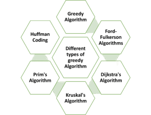
• Ford-Fulkerson Algorithms

The Ford-Fulkerson algorithm is a Greedy and Graph-based algorithm used to find the maximum flow in a flow network from a source node (s) to a sink node (t).

It works by finding augmenting paths in the residual graph and increasing the flow along these paths until no more augmenting paths are available.

Key Concepts:

• Flow Network: A directed graph where each edge has a capacity and carries a flow.
• Residual Graph: Shows the remaining capacity of edges after flow is applied.
• Augmenting Path: A path from source to sink where additional flow can be pushed.
• Bottleneck Capacity: Minimum capacity on an augmenting path (limits the flow you can add).

 Working (Step-by-Step):

1. Initialize all flows to 0.
2. While an augmenting path exists from s to t in the residual graph:
   • Find the minimum residual capacity (bottleneck) along the path.
   • Add this capacity to the flow of each edge in the path.
   • Update the residual graph accordingly (forward and reverse edges).
3. Repeat until no more paths are found.

Example:

Imagine a graph like this:

Source → A → Sink

   10     5

• Capacity of Source→A = 10
• Capacity of A→Sink = 5
• First augmenting path: Source → A → Sink
  Bottleneck = min (10, 5) = 5
  Flow is increased by 5.
  No more augmenting paths → Done.

 Maximum flow = 5

Ford-Fulkerson Algorithm (Max Flow) Python code:

def ford_fulkerson(graph, source, sink):

    max_flow = 0

    while True:

        path, flow = find_augmenting_path(graph, source, sink)

        if not path:

            break

        for u, v in path:

            graph[u][v] -= flow

            graph[v][u] += flow

        max_flow += flow

    return max_flow

Time Complexity:

• O (E × max_flow), where E = number of edges

 Advantages:

• Conceptually simple and powerful.
• Works on any graph with non-negative edge capacities.

Limitations:

• May not run in polynomial time if irrational capacities are used.
• Needs improvement (like using BFS in Edmonds-Karp) to ensure efficiency.

• Dijkstra’s Algorithm

Dijkstra’s Algorithm is a Greedy algorithm used to find the shortest path from a source vertex to all other vertices in a weighted graph with non-negative edge weights.

It works by repeatedly selecting the vertex with the minimum distance and updating the distances of its adjacent vertices.

Key Properties:

• Works only for graphs with non-negative weights
• Suitable for single-source shortest path
• Based on greedy choice of minimum distance

Step-by-Step Working:

1. Set distance of source node to 0 and all others to infinity.
2. Add all nodes to a priority queue or min-heap.
3. While queue is not empty:
   • Pick the node with the minimum distance.
   • For each neighbour, calculate new distance.
   • If new distance < old distance, update it.

Example Graph:

Vertices: A, B, C, D, E 

Edges: 

A → B (4), A → C (1) 

C → B (2), B → D (1), C → D (5), D → E (3)

Source: A

Shortest Path from A:

Dijkstra’s Algorithm (Shortest Path) python code:

import heapq

def dijkstra(graph, start):

    dist = {v: float(‘inf’) for v in graph}

    dist[start] = 0

    pq = [(0, start)]

    while pq:

        cost, u = heapq.heappop(pq)

        for v, weight in graph[u]:

            if dist[v] > cost + weight:

                dist[v] = cost + weight

                heapq.heappush(pq, (dist[v], v))

    return dist

Time Complexity:

• Using priority queue (heap): O((V + E) log V)

• Kruskal’s Algorithm

Kruskal’s Algorithm is a Greedy Algorithm used to find the Minimum Spanning Tree (MST) of a connected, undirected, and weighted graph.

It works by sorting all edges in ascending order of weight and adding the smallest edge to the spanning tree without forming a cycle, until the tree has (V – 1) edges.

 Key Concepts:

• MST: A tree that connects all vertices with the minimum total weight and no cycles.
• Uses Disjoint Set (Union-Find) to detect cycles.
• Greedy: Always picks the lightest available edge.

 Step-by-Step Working:

1. Sort all edges in non-decreasing order of weight.
2. Initialize each vertex as a separate component.
3. Pick the smallest edge and check if it forms a cycle using Union-Find:
   • If it doesn’t form a cycle, include it in the MST.
   • If it forms a cycle, skip it.
4. Repeat until (V – 1) edges are included in the MST.

Example Graph:

Vertices: A, B, C, D
Edges:

Sorted Edges: A-B (1), A-D (2), C-D (3), B-C (4), B-D (5)

Include: A-B, A-D, C-D
Final MST Edges: A-B, A-D, C-D
Total Weight = 1 + 2 + 3 = 6

Kruskal’s Algorithm (MST) python code:

def kruskal(edges, n):

    parent = list(range(n))

    def find(u):

        if parent[u] != u:

            parent[u] = find(parent[u])

        return parent[u]

    def union(u, v):

        parent[find(u)] = find(v)

    mst = []

    edges.sort()  # Sort by weight

    for weight, u, v in edges:

        if find(u) != find(v):

            union(u, v)

            mst.append((u, v, weight))

    return mst

Time Complexity:

• Sorting edges: O (E log E)
• Union-Find operations: O (E α(V)) ≈ linear time
• Total: O (E log E)

• Prim’s Algorithm

Prim’s Algorithm is a Greedy algorithm used to find the Minimum Spanning Tree (MST) of a connected, undirected, and weighted graph.

It starts from any one vertex and repeatedly adds the smallest-weight edge that connects a visited vertex to an unvisited vertex, expanding the MST one vertex at a time, until all vertices are included.

The algorithm ensures that the resulting tree:

• Includes all vertices
• Has no cycles
• Has the minimum possible total edge weight

 How It Works (Step-by-Step):

1. Start from any vertex (say, vertex A) and mark it as visited.
2. Add all edges connected to A into a min-heap (priority queue).
3. Pick the edge with the smallest weight from the heap.
4. If it connects to an unvisited vertex, add it to the MST and mark that vertex as visited.
5. Add all edges from the newly visited vertex to the heap.
6. Repeat steps 3–5 until all vertices are included and the MST has V − 1 edges.

Example:

Let’s take a graph:

Vertices: A, B, C, D 

Edges: 

A — B (1) 

A — C (3) 

B — C (1) 

B — D (4) 

C — D (2)

Steps:

1. Start from A → Add edges A-B (1), A-C (3) to heap
2. Pick A-B (1), add B to MST
3. From B, add B-C (1), B-D (4)
4. Pick B-C (1), add C
5. From C, add C-D (2)
6. Pick C-D (2), add D → All vertices included

Final MST Edges:

• A–B (1)
• B–C (1)
• C–D (2)

Total Weight = 1 + 1 + 2 = 4

Prim’s Algorithm (MST) Python code:

import heapq

def prim(graph, start):

    visited = set()

    min_heap = [(0, start)]

    total_weight = 0

    while min_heap:

        weight, u = heapq.heappop(min_heap)

        if u in visited:

            continue

        visited.add(u)

        total_weight += weight

        for v, w in graph[u]:

            if v not in visited:

                heapq.heappush(min_heap, (w, v))

    return total_weight

Time Complexity:

Where:

• V = Number of vertices
• E = Number of edges

Use Cases:

• Designing network cables, roads, or power grids with minimal cost.